The spectral analysis window opens when selecting the
DSP > Spectral Analysis menu.
If an audio track is available, the Fast Fourier Transform (FFT) is computed.
The first sample point of the data set used for computing the FFT is the cursor
position (red) in the active audio chanel window.
The blue cursor in the audio window shows the last sample point
(see Select an audio region).
The Size combo box controls the FFT sample size.
Available sizes are power of 2 integers and the corresponding frequency
resolution ("sample size"/"audio sample rate") is written beside each
value.
The Window combo box sets the FFT window type.
Available types are Rectangle, Triangle, Hann, Hamming , and Blackman.
Clicking on the button
Refresh the FFT taking into account current settings and cursor position.
The Offset checkbox allows to shift the FFT with a value set in the entry beside.
The next colored button opens a dialog box that allows you to set the
curve color and the entry beside, the curve width.
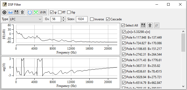
If LPC is checked, the Linear Predictive Coding coefficients are computed
with the same sample size than the FFT but always using a Hamming window.
The LPC order can be set with the entry beside.
Pole values and bandwidths are printed on the plot.
LPC can also be used to create DSP filters.
FFT and LPC spectrum obtained on a recorded vowel ɑ.
DSP Filters
The DSP Filter editor opens when clicking on the DSP > Filter menu.
It enables to design DSP filters as a cascade of individual filters.
Top toolbar
When clicking on the button, a filter
corresponding to the current setting (filter type and related entries) is added to the cascade
and a filter line is created in the right panel.
The button
exports both
selected and unselected filters.
⚠ The button
in the right panel exports only the
selected filters.
The button in the top toolbar
removes all filters.
The button applies the
cascade of active filters to the audio track.
The button
reverses time on the active audio track.
The ∂/∂t button replaces the active audio track by its time
derivative. The resulting signal is divided by its maximum absolute value so
that it is still an audio track bounded by [-1,1].
The maximum absolute value is printed as Norm Factor in the signal view.
The φ checkbox shows or hides the phase (arg(H))
view.
The RT checkbox enables Real Time filtering.
When checked, the current DSP
filter is applied in real-time while an audio track is playing.
⚠ The total size of the filter
(the sum of individual filter orders) that can be filtered in real time depends
on the computer performances. You may also need to increase your
Latency when using large order
filters for avoiding crackling.
If 0φ is checked, there will be no group delay
in the resulting signal.
If the filter is a FIR
(Kaiser Window filter or Equiripple),
the result signal is shifted by the half of the filter order.
If the filter is an IIR filter, the filter is applied two times:
one forward and one backward. In that case, the transfer function
is squared: H(f) => H2(f).
⚠ This option is
incompatible with Real Time.
The right panel
The button
exports only the
selected filters.
⚠ The button
in the top toolbal exports both
selected and unselected filters.
The Select All checkbox
select/unselect all filters below.
If a filter is checked ,
the filter is active. If it is unchecked , it is not
taken into account for
DSP computations.
The frequency response of the cascade filtering that is applied to the audio track
when clicking on the button
is plotted in the left view.
💡 A filter in the cascade can be a parallel filter
bank
whose content is displayed on mouse hovering.
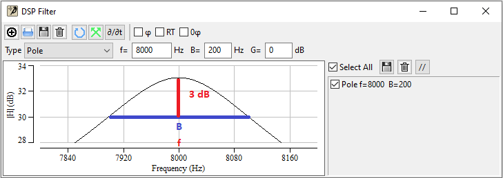
if the filter type is on Pole,
you can design a second order pole IIR filter by setting up
it center frequency f, its bandwidth B and a gain G.
A second order pole IIR filter defined by its frequency f and its bandwidth B.
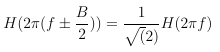
The bandwidth B is the width of the interval around the peak frequency
where the square amplitude is the half than the peak's one or
which is about 3 dB (20 log10(1/√ 2)).
The gain G if the transfer function module at null frequency: H(0).
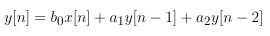
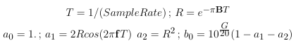
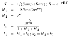
The difference equation for a second order pole IIR filter is
whose coefficients are obtained with the following relations:
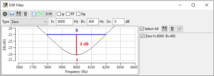
Zero
if the filter type is on Zero,
you can design a second order zero FIR filter by setting up
it center frequency f, its bandwidth B and a gain G.
A second order zero IIR filter defined by its frequency f and its bandwidth B.
The frequency f and gain G are defined as for the Pole,
the bandwidth B is the width of the interval around the bottom frequency
where the square amplitude is twice than the bottoms's one.
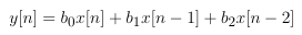
The difference equation for a second order zero FIR filter is
whose coefficients are obtained with the following relations:
Butterworth
Butterworth filters are designed to have a flat response
(no ripple) in the passband.
The design requirement is obtained with lower order than
FIR filters obtained by Windowing but they have
a non-linear phase that cause phase distortion.
The second combobox sets the filter shape. It can be lowpass,
highpass, band or notch.
A Butterworth low-pass IIR and high-pass filters are defined by a
cutoff frequency, f, an order, O and a gain G.
The O entry sets the filter order for low-pass and high-pass filter
orders but 1/2(filter order) for band-pass and notch filters.
The G entries sets the maximum value of the frequency responses.
Clicking on the Design button opens a dialog box that allows you to
design the filter in function of its passband (fp) and stopband (fs) edge frequencies and its
passband (Ap) and stopband (As) attenuations.
In the passband (f ≤ fp), we have |H(f)| ≥ -Ap,
and in the stopband (f ≥ fs), we have |H(f)| ≤ -As.
⚠ Design parameters must obey
As and Ap ∈ [0.01, 200], fs - fp ≥ 1 for the low pass
and fp - fs ≥ 1 for the high pass.
Butterworth pass band and notch IIR filters are defined by
a center frequency f, a bandwidth B, an order O
and a gain G.
The bandwidth determines the 3 dB attenuation around the center frequency.
Chebyshev
Chebyshev filters have a steeper roll-off than Butterworth filters, and have either passband ripple (type I)
or stopband ripple (type II).
If Type II is unchecked, it is a Type I Chebyshev filter
and δI is the passband ripple amplitude.
The second combobox sets the filter shape. It can be lowpass,
highpass, band or notch.
The O entry sets the filter order for low-pass and high-pass filter
orders but 1/2(filter order) for band-pass and notch filters.
The G entries sets the maximum value of the frequency responses.
The δI entry set the passband ripple amplitude.
For Type I low-pass and high-pass filters, the f entry
sets the cutoff frequency.
The Type I low-pass has a frequency response in the range 0-δI dB
between 0 and f.
The Type I high-pass has a frequency response in the range 0-δI dB between
f and the Nyquist frequency (0.5*sampleRate).
For band and notch filters, the f entry
sets the center frequency and the B entry the bandwidth.
The Type I band filter has a frequency response in the range 0-δI dB
between f - B/2 and f + B/2.
The Type I notch filter has a frequency response in the range 0-δI dB
between 0 and f - B/2 and between f + B/2 and the Nyquist frequency.
If Type II is checked, it is a Type II Chebyshev filter
and δII is the stopband ripple amplitude.
The O and G entries are the same
as Type I filters.
For Type II low-pass and high-pass filters, the f entry
sets the cutoff frequency.
The Type II low-pass filter has a frequency response below -δII dB
between f and Nyquist frequency (0.5*sampleRate).
The Type II high-pass filter has a frequency response below -δII dB
between 0 and f.
For band and notch filters, the f entry
sets the center frequency and the B entry the bandwidth.
The Type II band filter has a frequency response below -δII dB
between 0 and f - B/2 and between f + B/2 and the Nyquist frequency.
The Type II notch filter has a frequency response below -δII dB
between f - B/2 and f + B/2..
Kaiser Window FIR filter
As can be seen in the slideshow below, Kaiser Window
FIR filters have a linear phase (arg(H)) and therefore does not cause phase distortion.
Another available linear-phase filter is the equiripple FIR filter.
Available options are lowpass, highpass, band and notch.
Examples and descriptions are given in the slides below.
⚠ In this application, linear-phase filters are always
Type I FIR filters because they have no constraints on the transfer function boundaries. They have and even
order.
The relation between the stopband attenuation As and the stopband
deviation δs is given by:
As= -20 log10 δs ⇔ δs = 10 - As/20 and therefore, in our example:
δs = 10 - 40/20 = 0.01
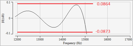
In the case of the Kaiser filter, the stopband deviation also sets
the limits of the ripples in the passband:
(1-δs) ≤ |H(f)| ≤ (1+δs)
∀ f ≤ fp
which in dB units gives:
|H(f)| ∊ [-0.0873 = 20*log10(0.99) ,
0.0864=20*log10(1.01)] ∀ f ≤ fp
Zoom on the ripples on the end of the pass band of the
low pass slide above (first one).
⚠ Since the design of the Kaiser filter depends on a parameter
that has
been determined empirically, it can occur that the requirements are not
almost fulfilled by the resulting filter and you could
have to adjust the stopband attenuation As in order to get the required filter.
⚠
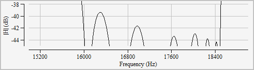
As can be seen in the figure below,
since a notch filter is obtained by the difference of two low pass
impulse responses, ripples of both filters are added and,
if the two stopband edges frequencties are close to each other
you may have to increase your stopband attenuation to meet the filter requirements.
The same remark is true for a bandpass filter by replacing stopband by passband
and difference by addition.
Zoom on the ripples of the stop band of the notch slide above (last one).
Comb Filter
Selecting the Comb type allows you to setup comb Filters
that can be used for artificial reverberation.
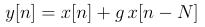
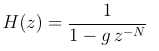
A comb filter is implemented by adding a delayed version of a signal to itself.
Two comb filter types are availaible: if the feedback
checkbox is unchecked it is a feedforward comb filter.
the Feedforward difference equation is
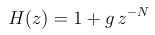
and the transfer function is given by
The gain parameter controls the depth and bandwidths
of the zeros. The two slides below show two transfer functions
with different values of g that must be smaller than 1.
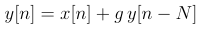
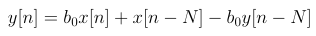
If feedback is checked, difference equation is
and the transfer function is given by
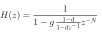
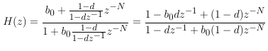
The delay line can be lowpass-filtered by multiplying the
z-N term by a first order pole transfer function.
The transfer function becomes (with a1=d and b0 = 1 - d)
If the damping parameter d is not 0, it controls the low pass filter
at the output of the delay line as shown in the third slide below.
⚠ if d < 0 or d > 1, some poles may be outside the unit cicle
and the filter is unstable (see Z-Domain view to check if poles are outside the
unit cicle).
As comb filters, allpass filters have been introduced by Schroeder for digital reverberation.
They have a flat frequency response amplitude.
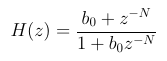
The difference equation is
and the transfer function is given by
As for the Comb Filter, the delay lines can be lowpass-filtered by multiplying
the
z-N term by a first order pole transfer function.
The transfer function becomes
that is no more an allpass filter since zeros are visible on the module of the transfer function.
⚠ if d < 0 or d > 1, some poles may be outside the unit cicle
and the filter is unstable (see Z-Domain view to check if poles are outside the
unit cicle).
It can be easier to generate long filter cascades using python scripts.
The last slide DSP filter can be obtained by copying the following python
code, save it as a .py file in your Macros directory
and load it from the application.
You can edit it in order to add or remove N values and modify the b0 and d parameters.
Several prime number tables are available on the internet
(e.g. widipedia).
                # some prime numbers

n_values = [127, 1223, 1373, 2137, 2473, 2837, 3163, 4021, 4523]

b0=0.98

d=0.05

DSPFilterOpen() # Open the DSP dialog

DSPClear() # Clear previous filters

for N in n_values:

    DSPFilterAllPass(N, b0, d)
Below is a small audio extract,
and here the result filtered with the cascade of 9 Schroeder allpass sections.
First Order IIR Filter
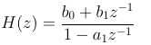
The difference equation for a first order
IIR filter is given by
y[n]= b0x[n] + b1x[n-1] + a1y[n-1],
and the corresponding transfer function is
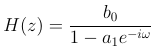
As example, for a First Order Pole low pass IIR filter (b1 = 0)
Since for a low pass filter, we want H(ω = 0) = 1, we must have a1 = 1- b0
as can be seen in the next slideshow.
If bw is checked as in the second slide below, instead of entering
the 3 coefficients b0, b1 and a1, you only have to enter
the 3 dB bandwidth that is the low pass cutoff frequency and a1 is calculated
using this equation.
⚠ The value you enter in this entry can be slightly modified because the
a1 coefficient is rounded to 6 decimal places.
In the second slide example, 200 is entered but the displayed value is 199.999.
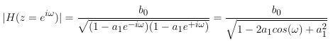
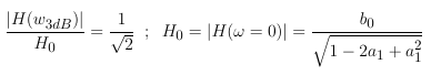
The magnitude of the frequency response is
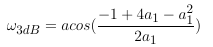
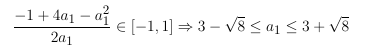
The 3 dB angular cutoff frequency is the ω3dB value for which
is given by
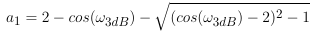
and a1 can be computed from ω3dB using
The corresponding frequency is ω3dB •
sampleRate/(2π).
💡 You can also use the first order filter to set up a Gain
by multiplying the input by a constant b0
(a1 = b1 = 0).
In dB unit, the gain is 20 log10(b0).
Linear Predictive Coding (LPC)
The Levinson-Durbin Recursion is used in order to get the LPC coefficients
from audio signal.
The inputs are the LPC order and the size of the sample used for LPC coefficients.
The start of the sample is the cursor position in the audio signal
view.
When clicking on the button, a
DSP filter corresponding to the coefficients is created.
If Inverse is checked, the inverse filter is obtaind: poles are converted to zeros
and the linear coefficient a0
becomes 1/a0. This can be used to extract the
glottal waveform from speech record.
If Cascade is checked, the filter is
decomposed into its poles and a gain (y[n]=a0x[n]).
Most are second order poles but first order poles whose frequency is 0 can be present.
IIR filter from LPC coefficients.
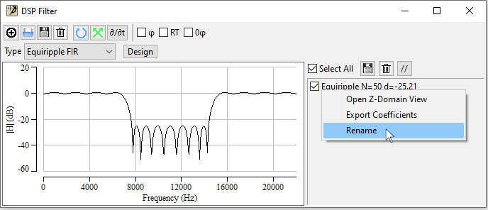
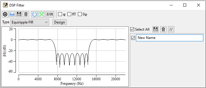
Rename
Right click on any filter in the right panel and select Rename
Enter the new name and then the Enter key for saving.
Type Esc for quitting without renaming.
z-domain View
Visualize any DSP filter poles and zeros in the z-domain plane.
⚠ The poles are the roots of denominator and the zeros are the roots of the
numerator of the the
transfer function.
The denominator and numerator are polynomials whose roots are obtained from the eigenvalues of a matrix
built with the polynomial coefficients.
The computation time is about O(nPoles3 + nZeros3).
As example, on an Intel core i7 processor running at 4.7 GHz,
the computation time is 0.7 sec for an all-zero filter of order 500, 8.36 sec if order is 1000
and 108.7 sec if the order is 2000.
Python
Here are the functions that can be called from Python scripts.
SoundFFTSetWindowType(string type) # set the FFT window type.
            SoundFFTDisplaySettings(int r, int g, int b, int hasOffset, float offset, int curveWidth)

 # r, g and b are the red green blue values for the

 # curve color (∈ [0,255]).
            curveWidth is the curve width.

 # If hasOffset != 0, offset if the curve offset.
            SoundFFTSetLPC(int b)

 # If b !=0, LPC is computed
            when SoundFFT() is called
SoundFFTSetLPCOrder(int order) # set the LPC order.
            DSPFilterType(string type) # set the DSP Filter Type

# Available types are: "Pole", "Zero",

# "Butterworth", "Chebyshev"

# "Kaiser Window", "Equiripple FIR", "Comb", "All Pass",

# "IIR 1st Order", "LPC" and "Import".
            DSPSelect(int i, int b)

# Select the ith filter available in the

# left panel of the DSP Filter dialog if b != 0,

# unselect it otherwise.

DSPDelete() # delete all selected filters.

DSPClear() # delete all filters.
            DSPFilterImport(string fileName)

# Import filter coefficients from file fileName.
            DSPFilterExport(std::string filterName, string fileName)

# Export the filter filterName coefficients
            to file fileName.
            DSPFilterRename(std::string oldName, string newName)

# Rename the filter oldName as newName.
            DSPFilterApply()

# Applies the current flter to the current audio track.
            SoundReverse()

# Reverse time of the current audio track.
            SoundDeriv()

# Replaces the current audio tract by its time derivative.
            DSPShowPhase(int b)

# Shows the phase in the DSP Filter dialog if b != 0,

# hides it otherwise.
            DSPApplyWhenPlay(int b) # ⚠ Deprecated: replaced by

DSPRealTime(int b)

# Activate Real Time if b != 0,

# deactivate it otherwise.
            DSPZeroPhase(int b)

# Activate 0-phase if b != 0,

# deactivate it otherwise.
            DSPOpenZView(string filterName)

# Open the Z-Domain View for the the filter filterName

# Returns view name
            GetDspSize();

#Returns the size of the DSP dialog box

#Example:  width, height = GetDSPSize()
            SetDSPSize(int width, int height)
            #Set the size of the DSP dialog box
            DSPFilterPole(float f, float b, float b)

 # Create a second order Pole at frequency f

 # with a bandwidth b and a gain g.
            DSPFilterZero(float f, float b, float b)

 # Create a second order Zero at frequency f

 # with a bandwidth b and a gain g.
            DSPFilterButterworth(string type, ....)

# if type is "low" or "hight", it creates a

# Butterworth Low Pass or High Pass  filter

 # and there must be 3 more arguments:

# cutoffFrequency (float) , order (int) and gain (float).


# if type is "pass", there must be 5 more float arguments:

# f1, A1, f2, A2, gain (A1 > 0, A2 > 0 and 0 < f1 <f2).

# This corresponds to settings the cutoff frequency

# and order from design paramenters.


# If A1 < A2, it is a low pass filter.

# f1 and f2 are the pass and stop frequencies.

# A1 and A2 are the passband and stopband attenuations.


# If A1 > A2, it is a high pass filter.

# f1 and f2 are the stop and pass frequencies.

# A1 and A2 are the stopband and passband attenuations.


# if type is "band" or "notch", there bust be 4 more arguments:

# centerFrequency (float), bandwidth (float),

# order (int) and gain (float).

# (see Butterworth Band Pass / Notch).
            DSPFilterChebyshev(int type, string shape, float cutoff, float delta, int order, float gain)
            # high-pass / low-pass

# Create a low-pass or high-pass Chebyshev filter

# type can be 1 for Type I chebyshev filter or 2 for Type II.

# shape can be "low" or "high" for low pass or high pass filter.

# cutoff is the cutoff frequecy.

# delta is the passband ripple amplitude if type is 1

# and the stopband ripple amplitude if type is 2.

# order and gain are the filter order and gain.
            DSPFilterChebyshev(int type, string shape, float center,float bandwidth,
            float delta, int order, float gain) # band-pass or notch

# Create a band-pass or notch Chebyshev filter

# type can be 1 for Type I chebyshev filter or 2 for Type II.

# shape can be "band" or "notch" for band-pass or band-stop (notch) filters.

# center is the center frequency.

# bandwidth is the filter bandwidth.

# delta is the passband ripple amplitude if type is 1

# and the stopband ripple amplitude if type is 2.

# order and gain are the filter order and gain.
            DSPFilterKaiser('lowPass', float fp, float fs, float As)

# Create a Low Pass Kaiser Window filter.

# with a passband frequency fp,

# a stopband frequency fs,

# and a stopband attenuation As (fp < fs)
            DSPFilterKaiser('highPass', float fs, float fp, float As)

# Create a Low Pass Kaiser Window filter

# with a stopband frequency fs,

# a passband frequency fp,

# and a stopband attenuation As (fs < fp)
            DSPFilterKaiser('band', fs1, fp1, As1, fp2, fs2, As2)

# Create a Band Pass Kaiser Window filter

# with a low stopband frequency fs1,

# a low passband frequency fp1,

# a low stopband attenuation As1,

# a high passband frequency fp2,

# a high stopband frequency fs2,

# and  a high stopband attenuation As2,
            DSPFilterKaiser('notch', fp1, fs1, As1, fs2, fp2, As2)

# Create a Notch Kaiser Window filter

# with a low passband frequency fp1,

# a low  stopband frequency fs1,

# a low stopband attenuation As1,

# a high stopband frequency fs2,

# a high passband frequency fp2,

# and a high stopband attenuation As2,
            DSPFilterComb(int b, int N, float g, float d)

# Create a Comb filter

# b=0 → feedforward; b != 0  → feedback

# N is the delay (in sample), g is the gain

# and d is the damping of the nested

# lowpass (only for feedback).
            DSPFilterAllPass(int N, float g)

# Create a Allpass filter

# N is the delay (in sample), g is the gain.
            DSPFilterFirstOrder(float b0, float b1, float a1)

# Create a First Order filter
            DSPFirstOrderLowpass(int b)

# Configure the first order IIR filter to be a low pass filter

# controlled by its 3dB cutoff frequency (check the bw checkbox)

# if b ≠ 0, uncheck it otherwise.
            DSPFilterLPC(int order, int size, int inverse, int cascade)

# Create a filter from LPC.

# inverse and cascade are considered as boolean.

# ⚠ An audio track must be available in the Audio GUI.
            ####################################################

# Functions that have no GUI equivalent.
            dsp_get_filter_list()

# Returns and array of filter names.
            dsp_get_num_filters()

# Returns the number of filters
            dsp_get_num_sub_filters(string filterLabel)

# Return the number of sub filters of filter filterLabel

# e.g. a Butterworth filter of order n is actually a cascade

# of n/2 filters of order 2
            dsp_get_coefficients(string filterLabel, in id)

# returns a and b coefficients of subfilter id for filter filterLabel.
Example: python script that exports all the filter coefficients in a File
filters=dsp_get_filter_list()
nFilters=len(filters) # could also be dsp_get_num_filters()
out_file=open("dsp_coefficients", "w")
for i in range(nFilters):
    label=filters[i];
    print("label:", label,file=out_file)
    # Number of sub filters. Both Butterworth
    # and Chebyshev are cascades of 2nd order IIR filters
    nSubFilter=dsp_get_num_sub_filters(label)
    for j in range(nSubFilter):
        a, b = dsp_get_coefficients(label,j)
        print("a=",a,file=out_file)
        print("b=",b,file=out_file)
        del a
        del b
del filters
 button
Refresh the FFT taking into account current settings and cursor position.
button
Refresh the FFT taking into account current settings and cursor position.

 button, a filter
corresponding to the current setting (filter type and related entries) is added to the cascade
and a filter line is created in the right panel.
button, a filter
corresponding to the current setting (filter type and related entries) is added to the cascade
and a filter line is created in the right panel.
 button
 button
 button in the top toolbar
removes all filters.
button in the top toolbar
removes all filters.
 button
reverses time on the active audio track.
button
reverses time on the active audio track.
 φ checkbox shows or hides the phase (arg(H))
view.
φ checkbox shows or hides the phase (arg(H))
view.
 button
copies the selected filters in a
button
copies the selected filters in a  , it is not
taken into account for
DSP computations.
The frequency response of the cascade filtering that is applied to the audio track
when clicking on the
, it is not
taken into account for
DSP computations.
The frequency response of the cascade filtering that is applied to the audio track
when clicking on the